Tree Traversal in Data Structure

Cheatsheet for Tree Traversal in Data Structures

Before learning about tree traversal in the data structure, let us first learn briefly about trees and their types.

The tree is a hierarchical non-linear data structure that is used to organize, store, and manipulated the data efficiently. As the name suggests, the data is stored in a tree-like structure. A tree data structure consists of various nodes (a node contains some data and a reference or a pointer that points to the other nodes).

Refer to the image for better visualization of the tree data structure.

As we can see in the image above, a tree data structure consists of a root node (the parent of all the other nodes) and a child node. The nodes which do not have any child node is known as a leaf node.

There are many types of tree data structures. Some of them are:

• Binary Trees
• Binary Search Trees
• B Trees
• B+ Trees
• AVL Trees
• Red-Black Trees
• N-ary Trees
• Splay Trees, etc.

Now, the tree traversal in the data structure is a technique that is used to traverse or visit the nodes of a tree (for printing, modifying, etc.). As we know all the nodes of a tree form a hierarchal structure (or we can say that they all are connected via edges), and we can easily traverse all the nodes using the root node or the head node. Using the root node, we can access every node of the tree if the tree is connected, but we cannot randomly select a node.

We have several tree traversal techniques available, let us learn about various tree traversal in data structure briefly.

In-Order Traversal

We first traverse the left subtree, then the root node, and finally the right subtree in the in-order tree traversal in data structure.

The pseudo-code for the in-order tree traversal in data structure can be:

Let us take an example tree to understand and visualize the in-order tree traversal in data structure better.

In the above tree, we will encounter node-1 first, since node-1 has a left subtree, we will recursively travel to the left sub-tree (consisting of node-2, node-4, and node-5). Again node-2 has left the child, so we will traverse to node-4. Now, finally, node-4 has no left or right child, we will print 4. After printing node-4, we will get back to node-2. Since all the left children of node-2 have been traversed, we can print node-2 as well. Similarly, we will get back to node-1 and print it.

Now, that all the left subtree of root node-1 has been traversed, we can continue the above algorithm on the right subtree.

Refer to the image to see the entire functioning of the in-order tree traversal in data structure.

The final in-order traversal obtained will be: 4 2 5 1 3.

Pre-Order Traversal

We first traverse the root node, then the lsubtreetree, and finally the right subtree in the pre-order tree traversal in data structure.

The pseudo-code for the pre-order tree traversal in data structure can be:

Let us take an example tree to understand and visualize the pre-order tree traversal in data structure better.

In the above tree, we will encounter node-1 first so we will print it. After this, we will move to the left subtree so we will traverse to node-2 and print it. Similarly, we will continue this process and recursively print the current node and traverse to the left subtree. After this, we will move on to the right sub tree and follow the same procedure.

Refer to the image to see the entire functioning of the pre-order tree traversal in data structure.

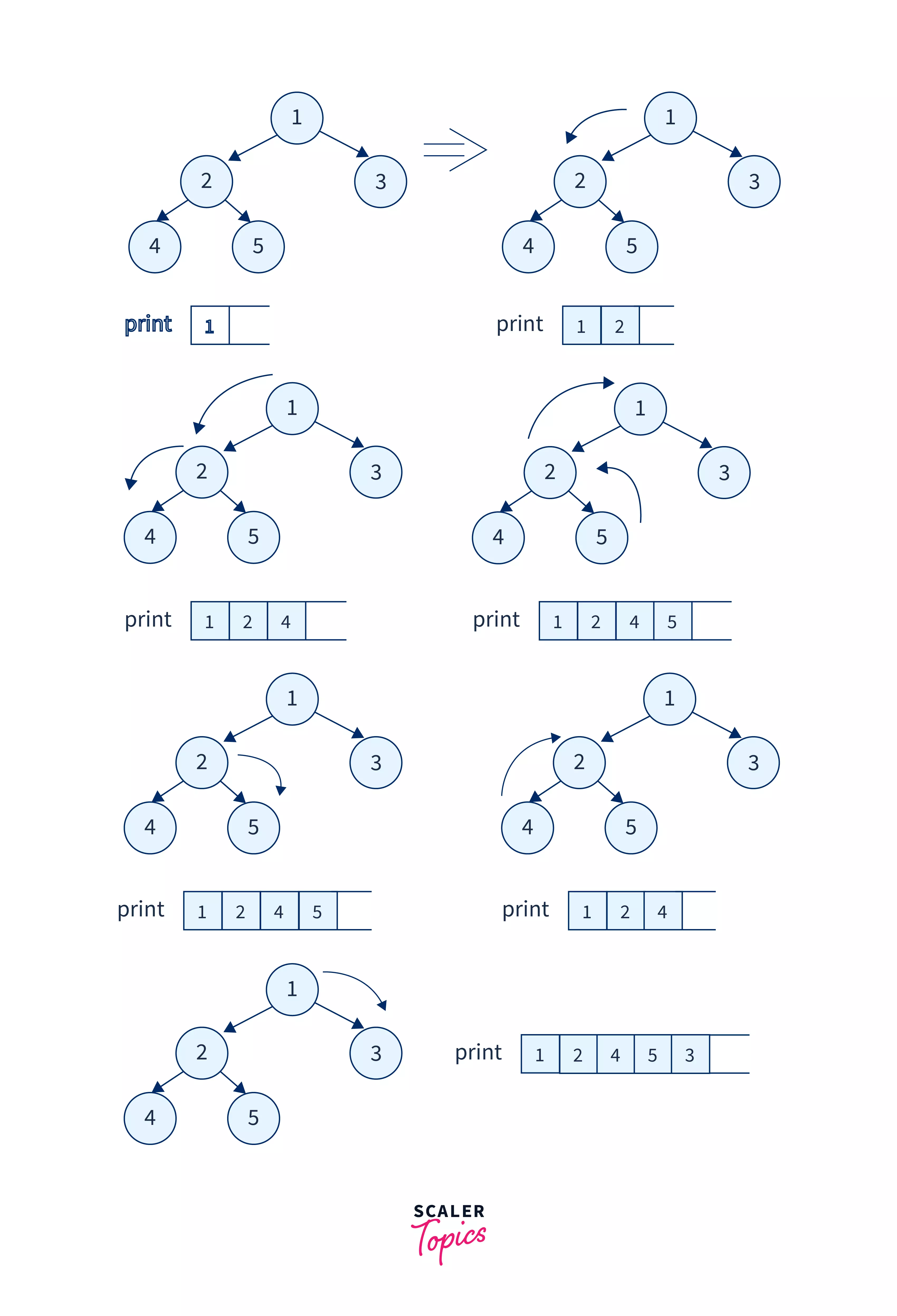
The final pre-order traversal obtained will be: 1 2 4 5 3.

Post-Order Traversal

We first traverse the left sub tree, then the right subtree, and finally the root node in the post-order tree traversal in data structure.

The pseudo-code for the post-order tree traversal in data structure can be:

Let us take an example tree to understand and visualize the post-order tree traversal in data structure better.

In the above tree, we will encounter node-1 first, since node-1 has a left subtree, we will recursively travel to the left sub-tree until there is no more left child available. When we get to node-4 (as there is no more left child), we will print it and move to the right subtree of the parent node i.e. node-2. So will be on node-5 and it will be printed. Similarly, we get back to the parent node and move to the right subtree. After traversing the left and right child, finally, we will print the parent node.

Refer to the image to see the entire functioning of the post-order tree traversal in data structure.

The final post-order traversal obtained will be: 4 5 2 3 1.

Level Order Traversal

In the level order tree traversal, the level of the root node is considered to be level-0 (in some explanations, you can find level-1 also). So, we first print the root node and then increase the level (i.e. we move through the depth). In this way we can print the entire tree. Generally the level order traversal is done using a queue data structure. Firstly we insert the root into the queue and iterate over the queue until the queue is empty. In every iteration, we will pop the front element of the queue and print its value. Then, we add its left child and right child to the end of the queue.

The pseudo-code for the level-order tree traversal in data structure can be:

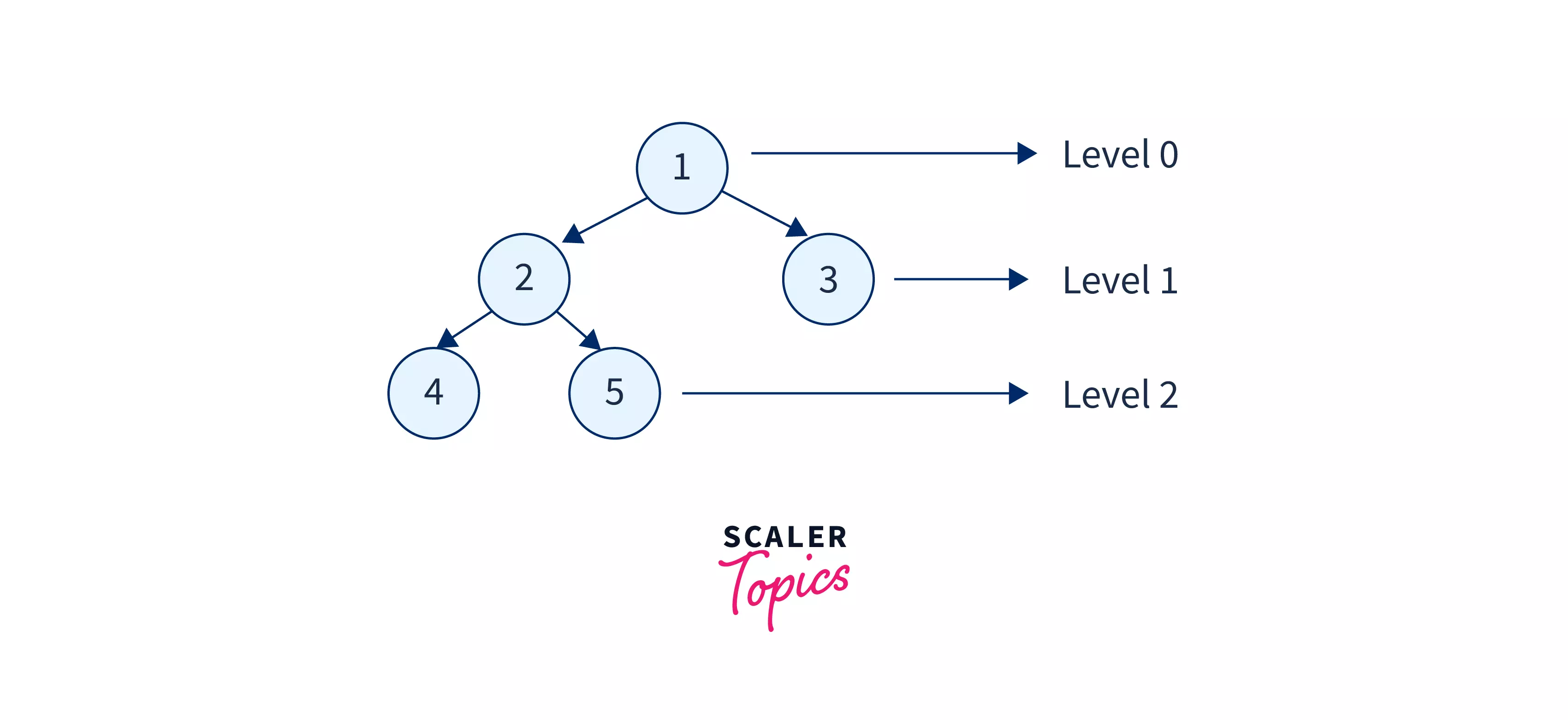
Let us take an example tree to understand and visualize the level order tree traversal in data structure better.

To learn more about the Level Order tree traversal in data structure, refer to the article: Level Order Traversal

In the above tree, we will encounter node-1 first, so we will print it. After printing the level-0 node i.e. node-1, we will increase the level as well as move to the next level and print the nodes of this level. Similarly, we will increase the level and print the nodes on the current level until the last node of the deepest level is traversed. We can use the queue data structuure to keep track of the levels.

The final level-order traversal obtained will be: 1 2 3 4 5.

DFS(Depth First Search)

DFS or Depth First Search uses backtracking for the tree traversal. Backtracking refers to trying out all the possible solutions and choosing the desired/best solutions. In the DFS, we start with a node and then taking a path from the chosen node, we go as deep as we can. Once we have found the deepest node (i.e. leaf node), we cannot go further using the same path so, we mark it visited and then backtrack to the parent node of the last visited node. We must go as deep as possible down one path before backing up and trying a different one.

Let us take an example tree to understand and visualize the Depth First Search tree traversal in data structure better.

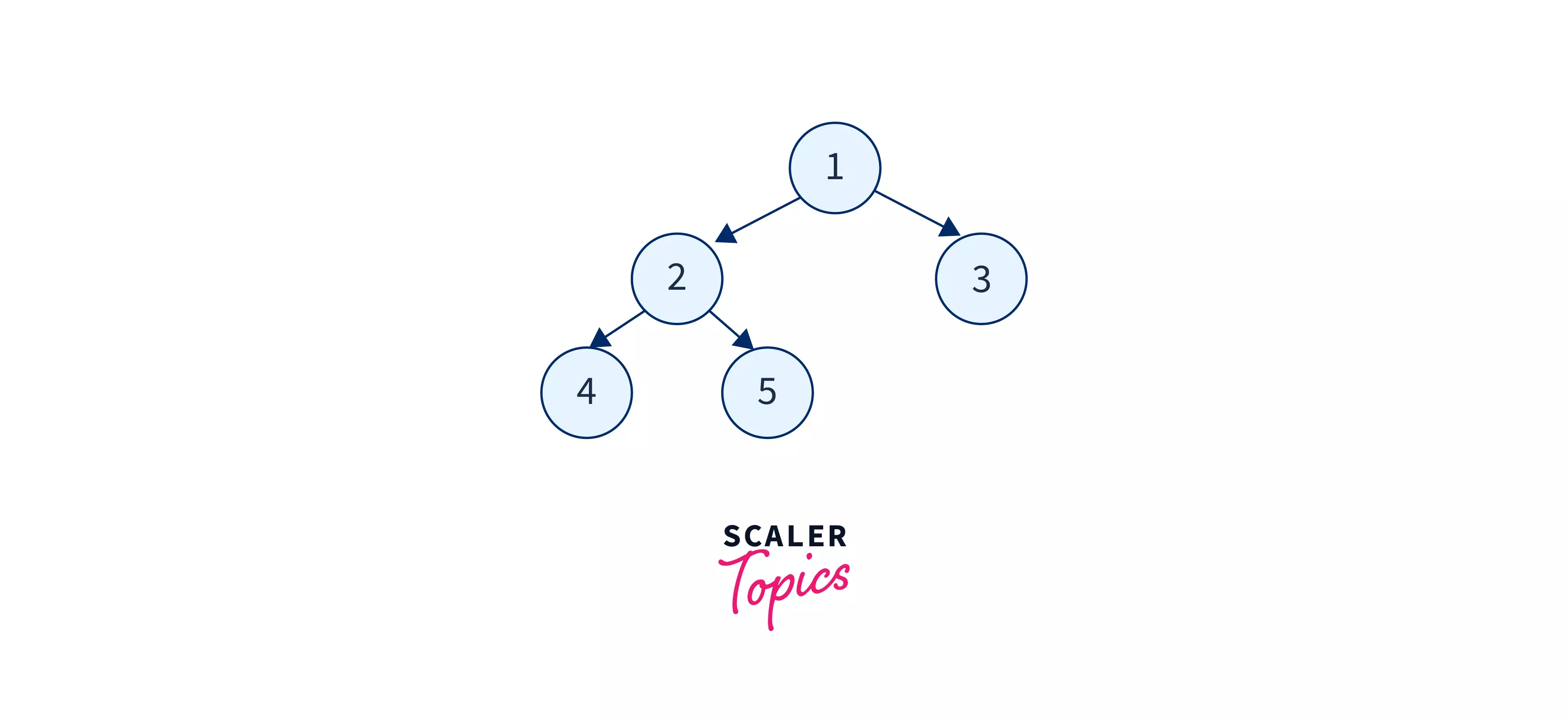
In the above tree, we will start with the root node i.e. node-1. We will start with this node, and print it. Now the node-1, we have two ways, we can choose either node-2 or node-3. Suppose we have chosen node-2 so we will print it and recursively call the function for the node-2. Again we can choose either node-4 or node-5. Suppose we have chosen node-4, so we will print it, and now since there is no way beyond node-4, we can backtrack. After backtracking, we will reach node-2, since the left child of node-2 is already traversed, we will move to the right child i.e. node-5. Similarly, we will traverse the entire tree.

Refer to the image to see the entire functioning of the DFS.

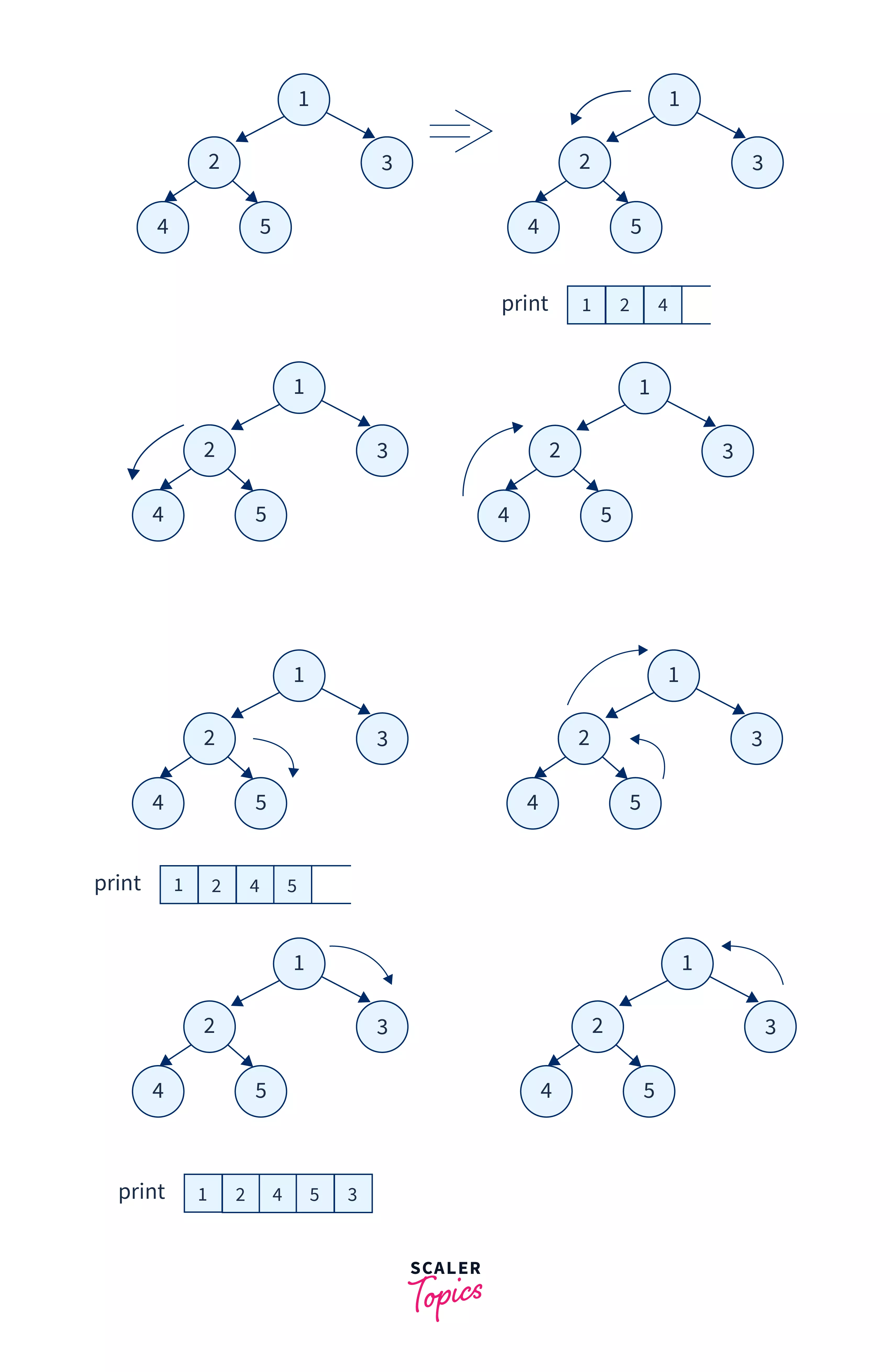
One of the depth-first search traversals obtained will be: 1 2 4 5 3.

To learn more about the Depth First Search and tree traversal in the data structure, refer to the article: Depth First Search (DFS) Algorithm

BFS (Breadth First Search)

BFS or Breadth-First Search is opposite the DFS. In the BFS instead of going deep into one path, we traverse all the direct paths related to the current node. So, we first traverse the current node and then traverses all the direct children of the current node. After all the direct children of the current root are traversed, we move to their children nodes and so on. It is somewhat similar to the level order tree traversal in data structure that we have studied earlier.

Let us take an example tree to understand and visualize the Breadth-First Search tree traversal in data structure better.

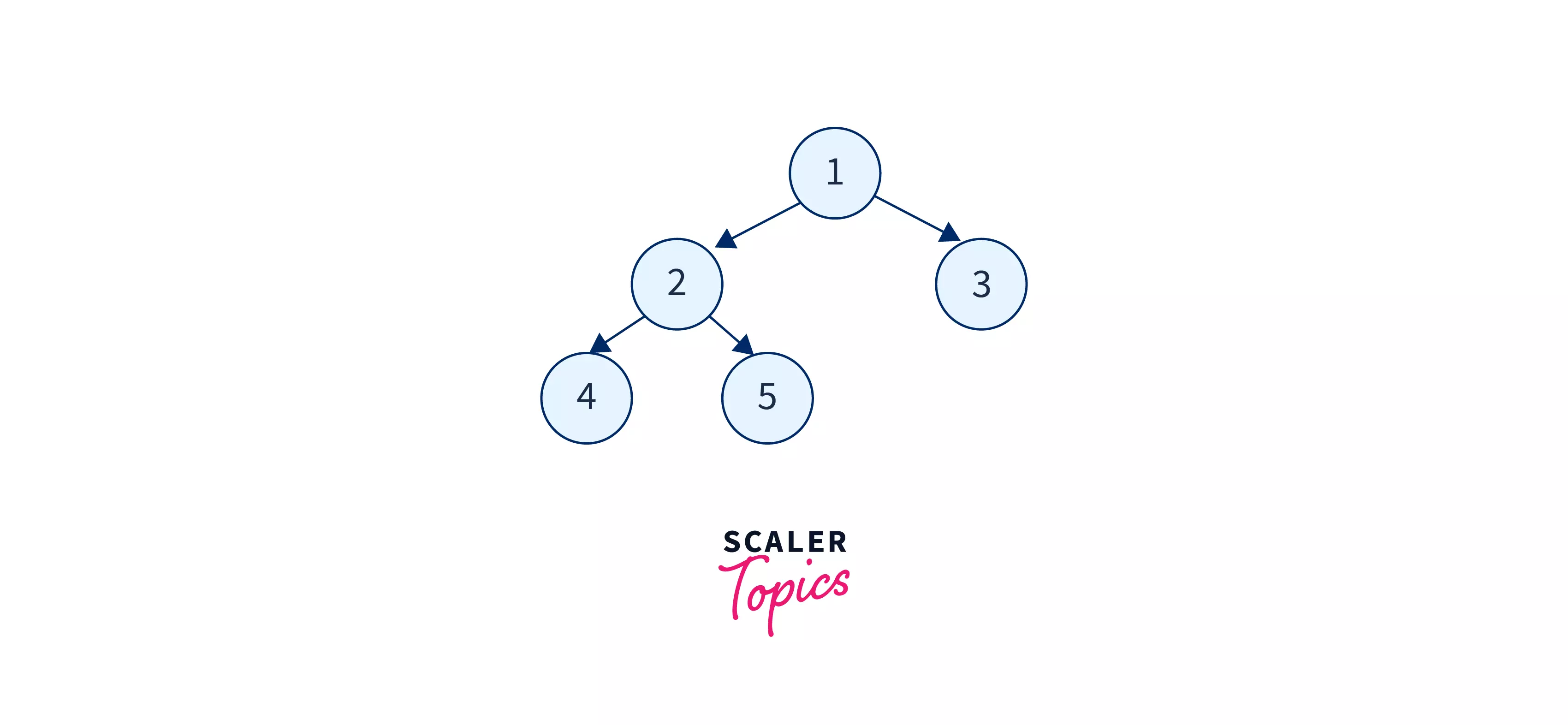
In the above tree, we will start with the root node i.e. node-1. We will start with this node, and print it. Now from node-1, we have two ways, we can choose either node-2 or node-3. So, we will print both the nodes i.e. 2 and 3. After printing them, we can move to node-2 and print all its child node(s). Similarly, we will traverse and print all the nodes of the tree.

The breadth-first search traversal obtained will be: 1 2 3 4 5.

To learn more about the Breadth-First Search and tree traversal in data structure, refer to the article: Breadth First Search | BFS

Complexity of Tree Traversal Techniques

Let us now learn about the time and space complexity of various tree traversal in the data structure.

1. In-order Traversal In the in-order traversal, we are traversing all the nodes once without using any extra space rather than the recursive stack call. Time complexity - O(n), where 'n' is the size of the binary tree. Space complexity - O(1).

2. Pre-order Traversal In the pre-order traversal, we are traversing all the nodes once without using any extra space rather than the recursive stack call. Time complexity - O(n), where 'n' is the size of the binary tree. Space complexity - O(1).

3. Post-order Traversal In the post-order traversal, we are traversing all the nodes once without using any extra space rather than the recursive stack call. Time complexity - O(n), where 'n' is the size of the binary tree. Space complexity - O(1).

4. Level order Traversal In the level order traversal, we are traversing all the nodes once. We are also using a queue data structure for the traversal. Time complexity - O(n), where 'n' is the size of the binary tree. Space complexity - O(n) because an auxiliary queue of size 'n' is used.

5. DFS (Depth First Search) In the DFS traversal, we are traversing all the nodes as well as we are using backtracking on the vistited nodes. We are also using a set or an array data structure for the traversal. Time complexity - O(E + N) [E is the edges and N is the number of nodes]. Space complexity - O(N) because an auxiliary visited array/set of size N is used.

6. BFS (Breadth-First Search) In the BFS traversal, we are traversing all the directly connectd nodes. We are also using a queue data structure for the traversal. Time complexity - O(E + N) [E is the edges and N is the number of nodes]. Space complexity - O(N) because an auxiliary queue of size N is used.