Fine-tuning an Image Classification Model in Keras

What are We Building?

This article will build a simple image classification Deep Neural Network Model. The image classification model will be trained on the MNIST-Fashion dataset and using the VGG-16 pre-trained layer as a base model. The classification model will comprise a VGG-16 pre-trained layer with weights of imagenet and our custom fully connected dense layer.

Pre-Requisites

Convolutional Neural Network (CNN)

A Convolutional Neural Network (CNN or convnet) is a subset of AI. A Convolutional Neural Network (CNN) is a type of network architecture for deep learning algorithms used for image recognition and other tasks requiring processing pixel data. In deep learning, there are other kinds of neural networks, but Convolutional Neural Networks are the preferred network architecture for identifying and recognizing objects. As a result, they are excellent candidates for applications requiring object recognition, such as self-driving cars and facial recognition, as well as computer vision (CV) tasks. for detail you can refer the here Dear Team Please add link of CNN article

TensorFlow and Keras

Keras is a compact, easy-to-learn, high-level Python library that runs on top of the TensorFlow framework. It focuses on understanding deep learning techniques, such as creating layers for neural networks, maintaining the concepts of shapes, and mathematical implementation.

Fine Tuning

Transfer learning is closely associated with fine-tuning. When we apply knowledge gained from solving one problem to a new but related issue, we experience transfer learning. For instance, a situation involving truck recognition could benefit from the knowledge gained from learning to recognize cars. One way to use transfer learning is through fine-tuning. More specifically, fine-tuning is the process of tuning or adjusting a model already trained for one task to perform another similar task.

How Are We Going to Build This?

The diagram below displays the flow of Fine-tuning the VGG-16 network on the MNIST-Fashion Dataset with a custom fully connected dense layer.

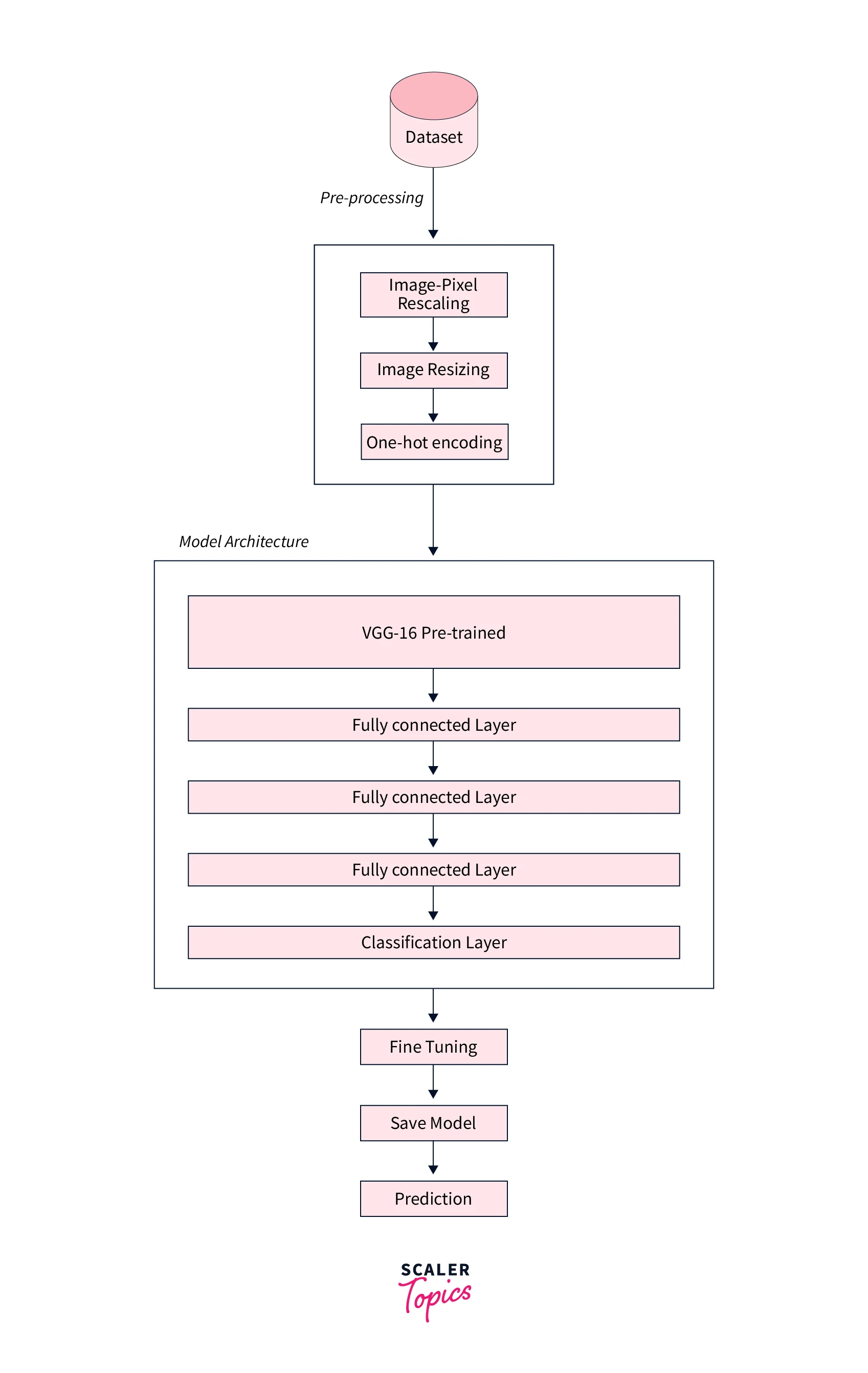
As we can see in the above image, there are five steps we are going to do so that we can accomplish our goal, i.e., fine-tuning the VGG-16 network, which is as follows:

1. Data Loading: In this part, we will load the Dataset from the Keras, which is already divided into Test and Train Dataset.
2. Data Preprocessing: For demonstration purposes, I have pre-processed the Dataset by resizing it and pixel rescaling, i.e., bringing the pixel value of the Dataset between 0-1.
3. Model Architecture: In this section, we will use VGG-16 pre-trained layer with a custom dense layer and a complete classification layer according to our Dataset.
4. Fine-Tuning: Fine-Tuning is an iterative process of deciding the hyper-parameter of the whole Dense Neural Network (DNN) as well as the pre-trained layers, i.e., to determine which layers we want to update the weights and backward propagate the weights which are dependent on the problem statement, Dataset and resources we have.
5. Save Model: Once the Model is trained, we need to save it from being used in real-time to make the Prediction. In this section, we will keep the Fine-Tuned Model so that it can be used to predict unseen data.
6. Prediction: Finally, we will predict the Test Dataset from the Model.

Final Output

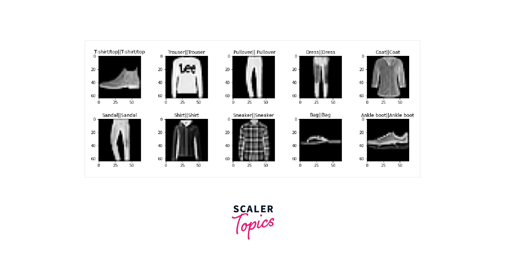
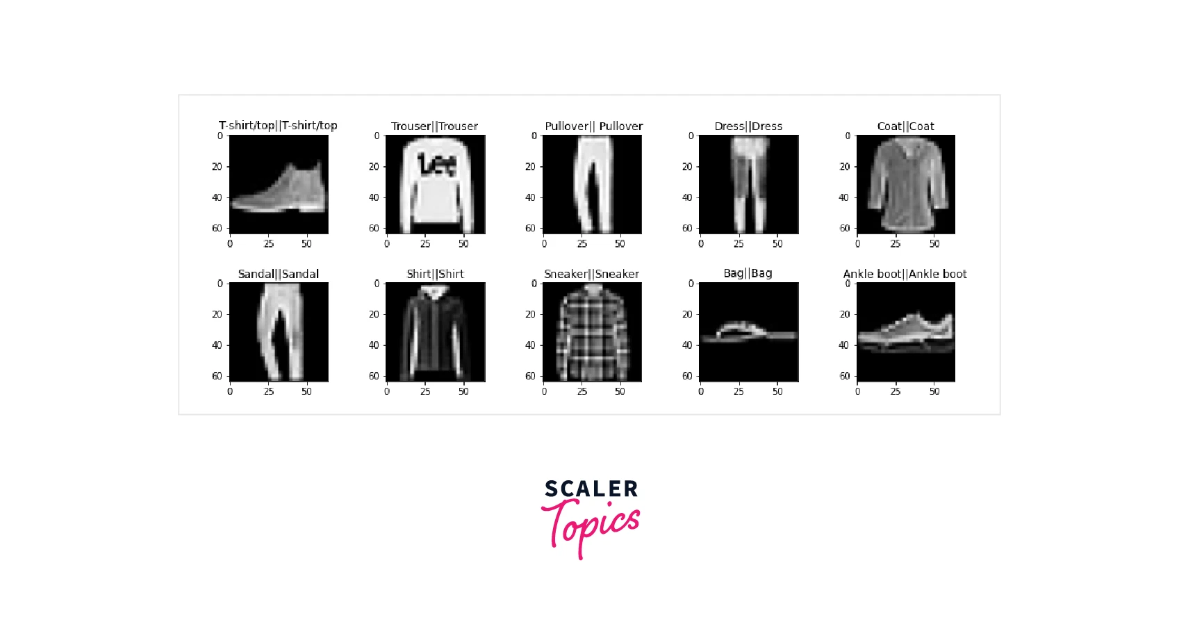
Classifying the object from images is one of the most important implementations of Artificial Intelligence because it mimics the human frontal lob and can function similarly to our eye. We have fine-tuned the VGG-16 to classify the objects. We trained the Model for one-epoch only, i.e., for demonstration purposes, and we obtained these metric value loss: 0.3377 - Accuracy: 0.8801 - val_loss: 0.2427 - val_accuracy: 0.9172. The below image shows the actual label || predicted label from the test set samples.

Requirements

A low-level set of tools to create and train neural networks is offered by Google’s TensorFlow2.x. With Keras, you can stack layers of neurons and work with various neural network topologies. We also use additional supporting packages like opencv2 and NumPy for data pre-processing. For the Dataset, we will be using MNIST-Fashion, available on the internet for free.

Fine Tuning an Image Classification Model in Keras

This is the essential part of this article. This section will discuss Fine-Tuning an Image Classifier Model in Keras. It is common knowledge that training convolutional networks requires significant data and resources.

All the Transfer Learning Models are trained on the Imagenet Data, which consists of 1000 objects and 14,197,122 annotated images. These pre-trained model weights are optimized for this Dataset only. Therefore, if we want to use the weights of these pre-trained models or even the architecture, in that case, we need to change the Model as per our requirement.

There are two approaches we can take:

1. Transfer learning: Remove the last fully connected layer from a ConvNet that has been pre-trained on ImageNet, and then treat the remaining ConvNet as a feature extractor for the new Dataset. Train a classifier for the new Dataset after extracting the features from all the images.
2. Fine-tuning: On top of the ConvNet, replace and retrain the classifier and use backpropagation to fine-tune the weights of the already trained network.

In this section, we will discuss the fine-tuning Image Classifier step by step and implement Transfer Learning on the VGG-16 Model with the MNIST-Fashion dataset, where the VGG-16 pre-trained weights will be updated as well as the Fully connected layer weight will be updated during the training process.

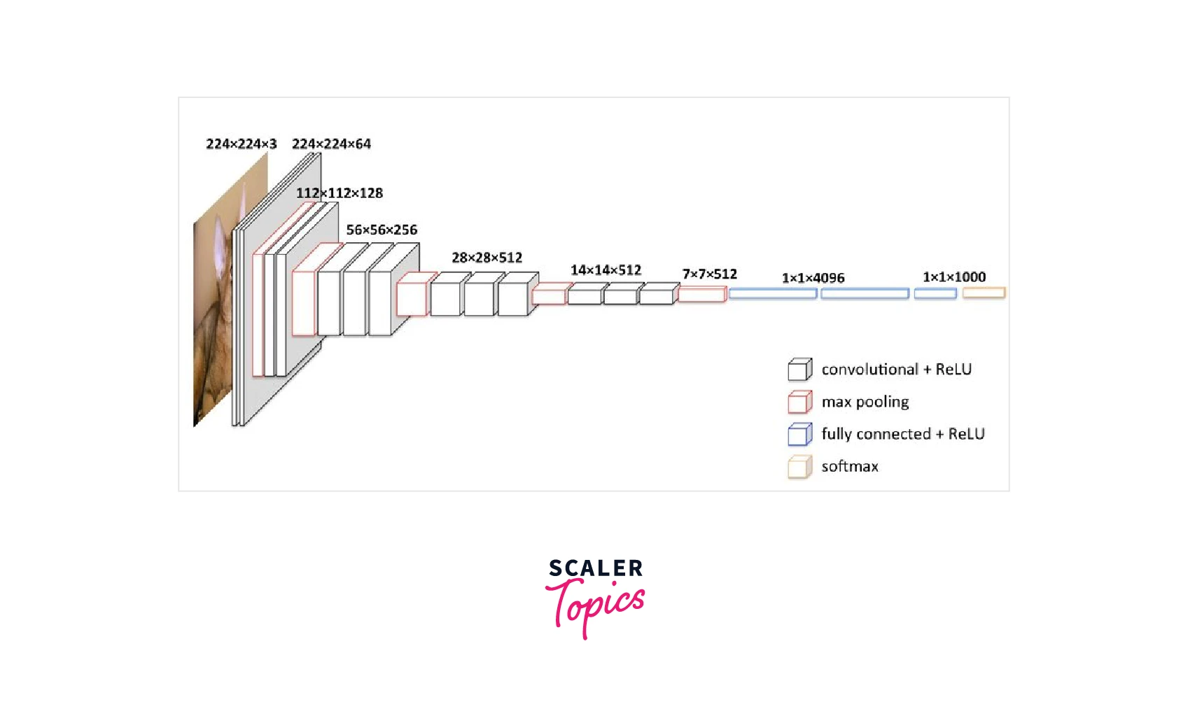
Model Architechture: As we already know, the number of neurons in the classification layer depends on the number of objects we want to classify. The pre-trained neural network is trained on the Imagenet Dataset, which consists of 1000 objects. Suppose the number of objects we want to class equals the number in the Imagenet Dataset. In that case, we can proceed as it is, but if the number of objects varies, we must implement our Dense Layer by the Dataset and optimes the weights of the Fully connected Layer only. The below image describes the VGG-16 architecture in depth:

Model Weights:

Weights are the backbone of any model. The training of the Model is the process of adjusting the weights so that the Model can predict correctly. The pre-trained Model is trained on Imagenet Dataset. So their weights are optimized or adjusted based on the Imagenet Dataset. If our Dataset is similar to the Imagenet dataset features, in that case, the same pre-trained weights will work as expected. Suppose our Dataset is not similar to the Imagenet. In that case, we need to optimize the weight again per our Dataset by setting the trainable parameter to True in the layers we want to optimize the weight. The below table describes the VGG-16 model layers and input/output shape in-depth:

Without further delay, let's get into the code right away. The data we used in the previous post will be used again. If you have a GPU, you can use a more extensive dataset because training on a CPU for a large dataset will take much longer. For fine-tuning, we will use the VGG-16 Model.

Step 1: Importing Required Libraries

The first step is to import the required libraries. Next, the snippets are used to import the required libraries for Keras so that the classes and functions can be implemented in our code along with the OpenCV library, which will be used to pre-process the Dataset.

Step 2: Data Loading and Data Preprocessing

For the explanation purpose, I have used the MNIST-Fashion dataset, which consists of 60,000 color images (composed of only one channel grey channel) of clothes bags, shoes, etc. The Dataset is divided into two sections, i.e., the Train set, which consists of 50,000 images, and the Test set, which consists of 10,000 images. I have also pre-processed the Dataset by normalizing and converting the labels into categorical values and reshaping the Dataset into 64,64,1 shape because we will implement the Convolution Neural Network 2D model. First, the Dataset is loaded from the Keras MNIST-Fashion dataset, which is already divided into training and testing sets. Then, the Dataset is scaled by dividing each pixel by 255 so that the value of each pixel is between 0 and 255 and reshaped into 64*64*3. The below code snippets depict the pre-processing steps of the MNIST Fashion dataset.

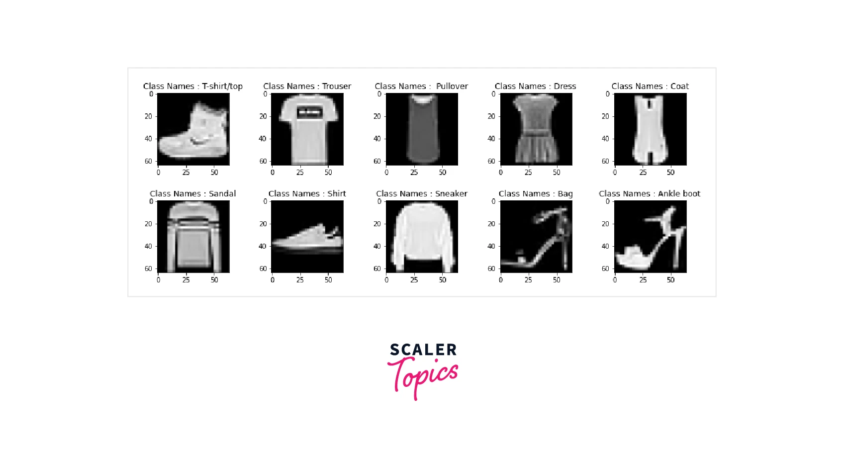
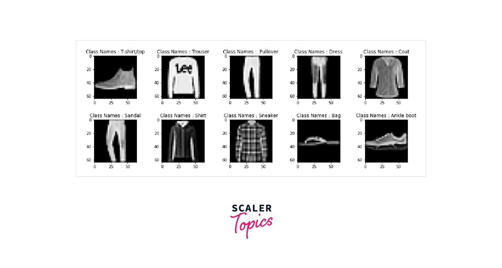
Step 3: Visualization of the Dataset

Data visualization is one of the essential parts of any Machine Learning (ML) / Deep Learning (DL) project. So, here I have visualized the Dataset using the matplot library.

I will plot 10 data samples from the training and testing dataset. I have created a subplot with two columns and five rows. I am extracting ten samples from the training dataset displayed along with its associated labels in the below code using the matplot library. The code snippets are shown below for the training and testing sets.

Step 4: Initiate VGG-16 Model

In this section, we will create a VGG-16 model without the top layer, i.e., we will remove the classification layer of the VGG-16 network.

In the below code snippets, I have specified the input shape of the input layer, i.e.,64*64*3, which is discussed in Step 2. Then we created the VGG-16 Model with pre-trained weights of imagenet and initialized the input_tensor parameter with the input layer. Also, we have specified that the classification layer of the Model should not be included in the Model by specifying include_top as False. Finally, I am showing the summary of the VGG-16 Model without a fully connected layer.

Each layer in Keras has a parameter called trainable.We should set this parameter to False to stop a particular layer from being trained and to freeze its weights. That’s all! After reviewing each layer, we decide which ones we want to train.

The model summary constitutes parameters trainable or non-trainable, layer name, and output shape of the layer. All the parameter of the VGG-16 is specified as trainable. The summary of the created Model is shown below:

Output

Step 5: Creating Fully Connected Layers

In the above step, i.e., in Step 5, we have created the VGG-16 Model without the Fully connected Dense Layer. But to solve the Classification problem, we need a fully connected layer with the number of neurons equal to the number of the object we want to classify. So we need to create a fully connected Dense Layer with the number of neurons in the Classification Layer equal to 10. The below code snippets are shown below:

As we can see in the above code snippets, I have implemented Flatten Layer because the output from the VGG-16 Model is in the shape of 2*2*512 2D- Tensor, but the Dense Layer accepts 1D Tensor. That is why I have implemented the Flatten layer to reshape the output of the VGG-16 into 1D Tensor. After the Flatten Layer, I have added 5 Dense Layers with the number of the neuron 1000, 800, 400, 200, and 100 along with the activation function relu. The last layer is the Classification Layer. It comprises the activation function known as Softmax, which outputs the probability of the classes associated with the datapoint and has a range between 0-1. This layer has ten neurons because we have to classify ten different objects.

Step 6: Creating Model

In this section, I will create a model which will be a combination of VGG-16 and our custom layer. The syntax for creating Models using tf.keras.Model is shown below:

As we can notice, the Model has parameters coming from VGG-16 set to trainable, whereas the parameter of the Fully connected layer is set to trainable. The model summary after combining the VGG-16 Model and our Model with VGG-16 and the Fully Classification Layer is shown below:

Output

Step 7: Model Compiling and Training

In the above step, we have created the Model. In this step, we will compile and train our Model. In this section, we are going to compile our Model. We must specify the loss function, optimizer, and metrics to compile the Model. I have used categorical_crossentropy as our loss function because our Dataset is multilabel. Adam was selected as the optimizer to propagate the error backward. Adam is an extension of the Stochastic Gradient Descent and a combination of the Root Mean Square Propagation (RMSProp) and Adaptive Gradient Algorithm (AdaGrad). We have used accuracy for simplicity; you can use any metric based on your problem statement. The below snippets depict the code for model compilation.

After successfully compiling the Model, our final step is to train the Model. The Dataset will be divided into two sets, i.e., training and testing sets. The argument validation_split denotes the ratio by which the Dataset will be divided. In our case, it is 0.1, which signifies that ten percent of the Dataset will be used for testing, and the remaining ninety percent will be used for training the Model with a batch size of 32. The below snippets depict the code for model training.

The model statistics for training over one epoch are shown below: Output

By default, the weight of the VGG-16 is set to Trainable =Ture, which means that the weights of VGG-16 will be updated or optimized during the whole training process. Only the weight of the Fully connected Dense Layer will be optimized

Step 8: Model Evaluation

Once the training of the Model is over, we need to evaluate our Model. The below code snippets depict the process for model evaluation:

As we can see, after training the Model only for one epoch, we have an accuracy of 0.8685 and a loss of 0.4654 shown below. Output

Step 9: Model Saving and Prediction

In this section, we will save the pre-trained Model and predict the Test dataset, unseen by the Model. We will select the test set as an input to the VGG-16 fined tuned image classifier model, and we will predict and finally display the result as shown below:

What Next?

In this article, we have fine-tuned the VGG-16 network on MNIST-Fashion, tried to fine-tune any other pre-trained model with the same Dataset, and compared the results. Also, you can extract the features from the pre-trained Dense Neural Network (DNN) and use that features to train any Machine Learning (ML) or Deep Learning (DL) model from scratch.